Smooth and Rough on the Highways of France

In a previous post I suggested that historians should use quantitative methods less to answer existing questions than to pose new ones. Such a digital humanities (DH) approach would be the reverse of the older social science history approach, in which social science tools were use to “answer” definitively longstanding questions. This post offers another example of how data visualization can suggest new questions, and how social science and humanistic methods can be complementary in unexpected ways.

One way to conceptualize this complementarity is John Tukey’s observation that “data = smooth + rough,” or, in more common parlance, quantitative analysis seeks to separate patterns and outliers. In a traditional social science perspective, the focus is on the “smooth,” or the formal model, and the corresponding ability to make broad generalizations. Historians, by contrast, often write acclaimed books and articles on the “rough,” single exceptional cases. These approaches are superficially opposite, but there is an underlying symbiosis: we need to find the pattern before we can find the outliers.

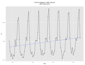
To highlight this complementarity, I pulled data on traffic on the French highway system from a blog on econometric methods. The data is clearly periodic, and for the blogger, Arthur Charpentier, the key question is how to model that periodicity. An autoregressive (AR) model? A moving average (MA) model? Autoregressive integrative moving average model (ARIMA)? Or maybe we should use spectral analysis to decompose the series into a collection of sine waves? These technical questions are important, and non-economists encounter these issues, if unwittingly on a daily basis when we read about “seasonally adjusted” inflation or unemployment.

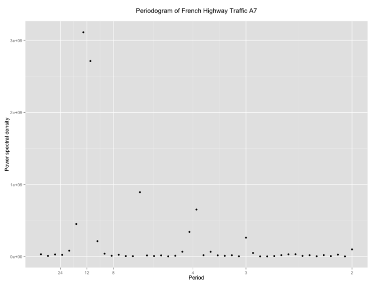
My quantitative/econometric chops are just good enough to enjoy experimenting with these methods, and while the details are complex, the core ideas are not. The graph below, a periodogram, shows that the traffic data has a strong “pulse” around the twelve-month mark and much smaller pulses around the four and three-month marks. There is a strong annual rhythm to the data, with several weaker seasonal pulses.

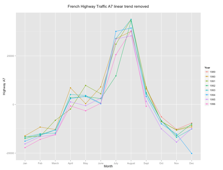
Now it’s great fun to play with sine waves, but as a DH historian, I would parse the data in different fashion. The periodogram, ironically, obscures the cultural aspects of periodicity. When exactly does traffic peak? Remapping the data confirms some conventional wisdom about France. Highway traffic peaks each year in July and August, as everyone heads to the forest or the beach. Yes, that’s why it seems like the only people in Paris in August are tourists.

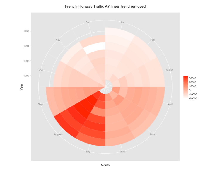
We can also visualize this annual cycle using polar coordinates, mapping the twelve months of the year as though they were hours on a clock, and visualize traffic volume with a heatmap, using darker colors for higher volumes of traffic. Kosara and Andrew Gelman had a valuable exchange on the merits of such visualizations, Kosara arguing in favor of polar coordinates and spirals, but Gelman noting the power of a conventional x-axis. It’s too rich for a quick summary—read their ideas!

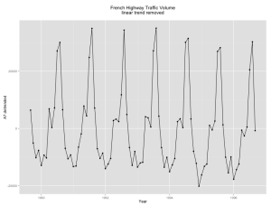
But from a DH perspective the most interesting thing about the data is not the trend, but the outlier. Look at the traffic for July 1992. It’s markedly below expectations. But then traffic was higher than average for August. What’s going on?

I let my freshman seminar students loose on the question and they quickly came back with an answer. The 1992 outlier corresponds to a massive truckers’ strike, sparked by a new system of penalties for traffic violations. Truckers blocked major highways for days and the French government deployed the army, which used tanks to clear the roads. The strike had an impact across the French economy and occupancy in vacation resorts dropped below 50%

It is here that social science and humanistic paradigms tend to part ways. For an economist, the discovery of the strike explains the outlier. She can delete that observation, or include a “dummy” variable and move on, satisfied that the model now better fits the data. There is more “smooth” and less “rough.” For a labor historian, this “rough” can become a research question. Why, of all the labor actions in the 1990s, was 1992 strike so striking in its impact? Was this a high water mark for French labor mobilization? Or did it inspire further actions? Did its impact on vacationers sour the general public on labor? And did the government back down on its regulations? For a historian, explaining this single outlier can be more important than understand any trend. The paradox is that the magnitude of outliers becomes clearer once we’ve modeled the trend, either visually or mathematically. The “drop” in traffic in July 1992 exists only relative to an expected surge in traffic. Thus, as I suggested in a previous post, historians need to build models and throw them away.

Leon Wieseltier writing about DH is like Maureen Dowd writing about hash brownies

What’s most striking about Leon Wieseltier’s essay in the New York Times Book review is how it confirms almost every cliché about the humanities as technophobic, insular, and reactionary. Not to mention some stereotypes about grouchy old men. Now I should confess at the outset to being a longtime Wieseltier cynic. His misreadings of popular culture always seemed mildly ridiculous. But what’s striking about the NYT piece is his vast ignorance of the subject. Wieseltier writing about digital humanities is like Maureen Dowd writing about hash brownies . Note to New York Times editorial writers: show a remote understand of the subject. Your ignorance is not a cultural crisis.

This line in particular, caught my eye: “Soon all the collections in all the libraries and all the archives in the world will be available to everyone with a screen.” Really? On what planet? Perhaps Wieseltier was thinking of this 1999 Qwest commercial for internet service?

Now I’m a specialist in Japanese history, and I’m certain that the millions of pages of handwritten early-modern documents in archives across Japan will not be all online “soon.” But even assuming that for Wieseltier “all the libraries” might mean modern publications in English, French and Hebrew, this is just nonsense. Has Wieseltier noted the metadata problems on Google Books? Or would understanding the limits to digitization be too much to ask?

What’s tragic about Wieseltier’s mindless opposition of the humanities versus technology it that it precludes exactly what we should be teaching: how to employ critical thinking when using technology. Dan Edlestein has a marvelous essay exploring how to search for the concept of “the Enlightenment.” His piece shows how, first, one can’t do a search without a basic understanding of the history of the Enlightenment itself, second, that quirky results are more than “mistakes.” Parsing weird and unstable search results can inform our understanding both of digital technologies and the history of ideas. The need for critical thinking in database searches actually proves the ongoing relevance of humanities in the internet age.

Of course, at the heart of Wieseltier’s panic is the “decline of the humanities.” Too bad Wieseltier doesn’t read the Atlantic. The humanities aren’t in decline. “The same percentage of men (7 percent) major in the humanities today as in the 1950s.” The overall drop over that period came from women, who began to pursue careers in the sciences because of the end of institutional gender bias. But that analysis came from the great digital humanities researcher Ben Schmidt. And understanding it would require taking both numbers and gender seriously. Which apparently is something great humanistic minds need not do.

Baseball, Football, Moneyball

In fall 2014 I taught a freshman seminar on data visualization entitled “Charts, Maps, and Graphs.” Over the course of the semester I worked with the students to create vizs that passed Tukey’s “intra-ocular trauma” test: the results should hit you between the eyes. Over the coming months I’ll be blogging based on their final projects.

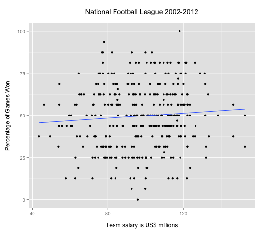
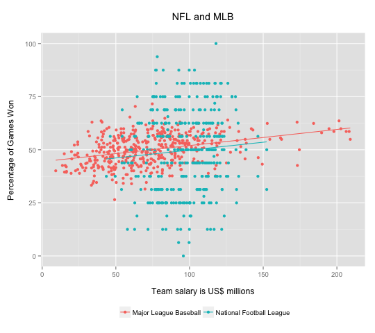
Today’s post is based on the work of Jeffrey You, who used US professional sports data, comparing baseball and football. As Jeffrey noted, the vizs highlight two key differences between the sports. First, the shorter football season (16 vs. 162 games per season) means that many football teams finish with the same record. The NFL scatterplot is therefore striated, and the winning percentage looks like a discrete variable. In fact there are limited outcomes for both baseball and football, but 162 possibilities looks continuous while 16 does not.

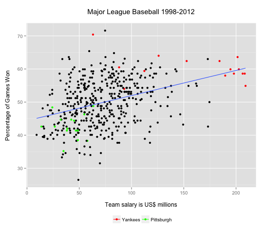
The other contrast is relative importance of total payroll in baseball. In neither case is there a strong correlation, but football is astonishingly low: r= 0.07 for the NFL compared to r=0.37 for MLB. What’s going on? Jeffrey suspected that injuries might play a greater role in the NFL, so a high payroll might pay for less actual playing time. He noted as well, the greater importance of single player. Tom Brady, he noted, was a 199^th draft pick with a starting salary of “only” $375,000.

The graphs also highlight the greater payroll range in MLB compared to the NFL. The regression line for MLB suggests that increasing a win-loss record by one game costs about $8 million. But the payroll spread in MLB so large that it can become a dominant factor. Jeffrey noted that for 2002-2012 the average payroll for the Yankees was $162 million while that of the Pirates was merely $41 million. For that same period, the Yankees have never won less than 50% of their games while the Pirates never won more than 50%. There is no comparable phenomenon for football. The standard deviation for MLB payrolls is about $35 million but for the NFL it’s less than $20 million.

NB: Technically, one should use the log of the odds rather than use winning percentage as the dependent variable, but in this case the substantive results are the same. For MLB the values range from 25% to 75%, in the more linear range of a logit relations. For NFL, there’s no appreciable correlation in either a linear or a logit model.

Fearbola, Ebola and the Web

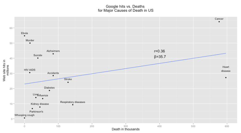
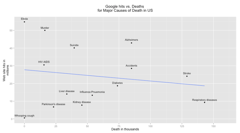
My nasty “cold” has been diagnosed as Influenza A, so it’s bed rest for 48 hours. And, of course, blogging about why Ebola gets all the news but not good ‘ol killers like influenza. I got CDC figures for deaths and then ran Google searches for the related terms, totaling the number of hits. I was surprised at first. The number of hits seemed to roughly correspond to the death rate. Ebola was way off, massively over reported, but the general trend seemed right. However . . . .

But that’s just an artifact of cancer and heart disease, which kill four times as many Americans as the “runner up,” respiratory diseases.

Once we remove these two, the data shows what I was looking for: presence on the web and mortality have no discernable relationship. In fact, the weak correlation is negative. Respiratory diseases are the number one killer after the cancer and heart disease, but they are not, it seems, web savvy. Same for kidney disease. Anyone have a t-shirt from the “Nephrotic syndrome 5K and Fun Run”? Didn’t think so. And don’t get me started on the flu, the Rodney Dangerfield of infectious diseases. In some cases, the abundance of websites makes sense. HIV AIDS transmission has plummeted becasue of public education. But why is Alzheimer’s a web sensation, whereas stroke is ho-hum? And, in some cases, these mismatches point to dangerous pubic confusion about risk. Heart attacks are considered a “man’s problem” but it’s a major cause of death for women. The relatively weak web presence of heart disease probably flags this gendered misperception, which then leads to the under-diagnosis and under-treatment of women.

Name	Web hits	Deaths	Web search term	CDC term
Ebola	54,800,000	1	Ebola deaths US	Ebola
Whooping cough	549,000	7	Whooping cough deaths US	Whooping cough
HIV AIDS	30,500,000	15,529	HIV AIDS deaths US	Human immunodeficiency virus (HIV) disease
Murder	50,000,000	16,238	Murder deaths US	Assault (homicide)
Parkinson’s disease	6,760,000	23,111	Parkinson’s disease deaths US	Parkinson’s disease
Liver disease	14,050,000	33,642	Liver disease deaths US	Chronic liver disease and cirrhosis
Suicide	40,100,000	39,518	Suicide deaths US	Intentional self-harm (suicide)
Kidney disease	7,780,000	45,591	Kidney disease deaths US	Nephritis, nephrotic syndrome, and nephrosis
Influenza Pnuemonia	13,350,000	53,826	Influenza deaths US PLUS Pnuemonia deaths US	Influenza and Pneumonia
Diabetes	18,700,000	73,831	Diabetes deaths US	Diabetes
Accidents	28,500,000	84,974	Accidents deaths US	Accidents (unintentional injuries)
Alzheimers	42,900,000	84,974	Alzheimer’s deaths US	Alzheimer’s disease
Stroke	24,100,000	128,932	Stroke deaths US	Stroke (cerebrovascular diseases)
Respiratory diseases	9,310,000	142,943	Respiratory disease deaths US	Chronic lower respiratory diseases
Cancer	64,100,000	576,691	Cancer deaths US	Cancer
Heart disease	27,200,000	596,577	Heart disease deaths US	Heart disease

 

 

Foodies, sushi, and Google Ngrams

Playing around with the new ngramr package for R, I came up with a simple viz for both the sushi boom and the rise of US foodie culture. Sometime a picture is worth a thousand words, but a least sushi is low in calories.

 

In praise of “Shock and Awe”

Why graph? And why, in particular, use innovative and unfamiliar graphing techniques? I started this blog without addressing these questions, but a recent blog post by Adam Crymble, critical of “shock and awe” graphs made me realize the need to explain EDA (Exploratory Data Analysis) and data visualization. Crymble wisely challenged data visualization practitioners to ask themselves the following questions: “Is this Good for Scholarship? Or am I just trying to overwhelm my reviewers and my audience?” This is sound advice, and Crymble’s concerns strike me as genuine. But, upon reflection, his post led me to think that “shock and awe” are evitable parts of any bold scholarly intervention. Feminist scholarship provoked genuine anger when it asserted that academic conventions were rife with sexist assumptions. The linguistic turn alarmed traditional scholars with its new understandings of literary production. Certainly these interventions produced (and continue to produce) needlessly complex, derivative prattle. But can anyone seriously argue that the humanities are not richer for these intellectual challenges?

What follows, therefore, is a defense of “shock and awe”: a justification for data visualizations that are unfamiliar, challenging, and demand news ways of thinking.

Why graph instead of just showing the numbers?

By just “show the numbers,” humanities researchers often refer to tables. The problem with this preference for tables it that is assumes that tables are somehow more transparent and accessible than graphs. In fact, the opposite is true.  A list of data values is like a phone directory: a wonderful way to look up individual data points, but a terrible means of discerning or discovering patterns. (Kastellec and Leoni 2007; Gelman, Pasarica, and Dodhia 2002) Alternately, a table of individual data points is analogous to collection of primary text sources: it’s the raw material of research, not research. Further most published tables are not transparent, “raw” data. On the contrary, tables in most research consolidate observations into groups, listing, for example, average wages for “skilled craftsman in Flanders 1830-35,” or “Osaka dyers 1740-80.” But why those years ranges and those occupational categories? Why 1830-35 instead of 1830-1840? Why Osaka dyers and not the broader category of Osaka textile workers? Those groupings may be conceptually valid, but they are interpretative and preclude other interpretations. Certainly we can lie with graphs, but we can also lie with tables. And since a good graph is better than the best table, DH researchers need to use good graphs.

Why these novel, unfamiliar graphs?

The data visualization movement has certainly produced some bad graphs —obfuscating rather than illuminating. But it is impossible to argue that newer graph forms are more misleading than the status quo. The pie chart, for example, is easy to misuse and the many variants supported by Excel are simply awful. With a 3D exploding pie chart, even a novice can make 5% look larger than 10% or even 15%. Can you correctly guess the absolute and relative sizes of the slices in this graph? 

(See answers below).  Since pie charts are familiar, they are accessible, but that simply makes them easier to misuse. Are conventional bad graphs such as pie charts “better” than newer chart forms because they provide easier access to faulty conclusions? Is “schlock” worse that “shock”?

My survey of graphing techniques in history journals tuned up an alarming result. Historians rely primarily on graphing techniques developed over 200 years ago: the pie chart, bar chart, and line chart. It is hard not to shock the academy with strange graphs, when “strange” means anything developed in the past two centuries. Many new graphing techniques, such as parallel coordinate plots, are still controversial, difficult to use, and difficult to interpret. But many others are readily accessible and widely used, except in the humanities, The boxplot, developed in 1977 by John Tukey, is now recommended for middle school instruction by The National Council of Teachers of Mathematics. The intellectual pedigree of the boxplot is beyond question: Tukey, a professor of statistics at Princeton and researcher at Bell Labs, is widely considered a giant in 20^th century statistics. So, what to do when humanities researchers are flummoxed by a boxplot? I now append a description of how to read a boxplot, but isn’t it an obligation of quantitative DH to push the boundaries of professional knowledge? And shouldn’t humanities Ph.D.’s have the quantitative literacy of clever eighth graders? In short, since our baseline of graphing skills in the humanities is so outdated and rudimentary, there is no avoiding some “shock and awe.”

A graph in seven-dimensions? What are you talking about? You must be trying to trick me!

Certainly “seven dimensions” sounds like a conceit designed to confuse the audience, or intimidate them into acquiescence. But a “dimension” in data visualization is simply a variable, a measurement. Decades ago Tufte showed how an elegant visualization, Menard’s graph of Napoleon’s invasion of Russia, could show six dimension on a 2D page: the position of the army (latitude and longitude), size of the army, structure of the Russian army, direction of movement, date, and temperature. Hans Rosling’s gapminder graphs use motion to represent time, thereby freeing up the x-axis. By adding size, color and text, Rosling famously fit six dimensions on a flat screen: country name, region, date, per capita GDP, life expectancy, and total population. These are celebrated and influential data visualizations, the graphic equivalents of famously compelling, yet succinct prose. While Crymble assumes that needlessly complex graphics stems from bad faith (a desire to intimidate and deceive), I am more inclined to assume that the researcher was reaching for Menard or Rosling but failed.

“How do you know there hasn’t been a dramatic mistake in the way the information was put on the graph? How do you know the data are even real? You can’t. You don’t.”

 

This concern strikes me as overwrought and dangerous. Liars will lie. They will quote non-existent archival documents, forge lab results, and delete inconvenient data points. When do we discover this type of deceit? When someone tries to replicate the research: combing through the archives, running a similar experiment, or trying to replicate a graph. How are complex graphics more suspect, or more prone for misuse than any other form of scholarly communication? Is there any reason to be more suspicious of complex graphs than any other research form?

I can optimistically read Crymble’s challenge as a sort of graphic counterpart of Orwell’s rules for writers. But Crymble seems to view data viz as uniquely suspect. To me this resembles the petulant grousing that greeted Foucault, Derrida, Lyotard, Lacan, etc some three decades ago – “what is this impenetrable French crap!” “You’re just talking nonsense!” Certainly many of those texts are needlessly opaque. But much of it was difficult because the ideas were new and challenging. The academy benefitted from being shocked and awed. Data visualization can and should have the same impact. The academy needs to be shocked — that how change works.

Gelman, Andrew, Cristian Pasarica, and Rahul Dodhia. 2002. “Let’s Practice What We Preach: Turning Tables into Graphs.” The American Statistician 56 (2): 121-30.

Kastellec, Jonathan P., and Eduardo L. Leoni. 2007. “Using Graphs Instead of Tables in Political Science.” Perspectives on Politics 5 (4): 755-71.

The pie chart:

Apple	10
Borscht	17
Cement	13
Donut	20
Elephant	25
Filth	15

Where the monks are(n’t)

After reviewing a book on religion in 19^th century Japan, I became curious about the quantitative dimension of religious practice, particularly the persecution of Buddhism. My initial visualizations turned into a exploration of how to visual spatial variation.

The 1871 census data reported two types of religious practitioners (monks and priests) totaled by either domain or prefecture. The data show a striking regional trend. The boxplot below shows the percentage of religious practitioners described as monks. In the Kinai, the median was about 80%. At the periphery, however, the percentage of monks was much lower: in Kyūshū, Chūgoku, Shikoku and Tōhoku the median was about 50%. The highest values for Kyūshū and Chūgoku are still below the median for the Kinai. Chūbu shows the most striking range, Naegi reporting 0% monk and Katsuyama 99%

The map below plots the extreme values for religious affiliation: domains with more 80% monks are marked as red, while less than 50% are marked in blue. Here again, we can see the same pattern – lot’s of monks around Kyoto and Nara, but fewer in Kyushu and the northeast. Two domains famous for their persecution of Buddhism, Mito and Kagoshima, are both in red, but so are nearby domains. What explains this regional trend  in religious practice?

Welcome to clioviz

What is clioviz? A blog devoted to data visualization in history and the humanities. What’s data visualization? An interdisciplinary approach to graphics that seeks to make trends and patterns in quantitative data visually apparent. In a well-designed data viz, patterns jump out at the viewer/reader, and results are obvious without the use of descriptive statistics. This blog grew out of an Emory graduate seminar (HIST 582 Quantitative Methods) and the initial posts come from those seminar papers. But we’ll be adding later work too, and linking to other sites/blogs in data viz and digital humanities.

Most of the viz’s here were produced in R, the language and environment for statistical computing and graphics