Smooth and Rough on the Highways of France

In a previous post I suggested that historians should use quantitative methods less to answer existing questions than to pose new ones. Such a digital humanities (DH) approach would be the reverse of the older social science history approach, in which social science tools were use to “answer” definitively longstanding questions. This post offers another example of how data visualization can suggest new questions, and how social science and humanistic methods can be complementary in unexpected ways.

One way to conceptualize this complementarity is John Tukey’s observation that “data = smooth + rough,” or, in more common parlance, quantitative analysis seeks to separate patterns and outliers. In a traditional social science perspective, the focus is on the “smooth,” or the formal model, and the corresponding ability to make broad generalizations. Historians, by contrast, often write acclaimed books and articles on the “rough,” single exceptional cases. These approaches are superficially opposite, but there is an underlying symbiosis: we need to find the pattern before we can find the outliers.

To highlight this complementarity, I pulled data on traffic on the French highway system from a blog on econometric methods. The data is clearly periodic, and for the blogger, Arthur Charpentier, the key question is how to model that periodicity. An autoregressive (AR) model? A moving average (MA) model? Autoregressive integrative moving average model (ARIMA)? Or maybe we should use spectral analysis to decompose the series into a collection of sine waves? These technical questions are important, and non-economists encounter these issues, if unwittingly on a daily basis when we read about “seasonally adjusted” inflation or unemployment.

My quantitative/econometric chops are just good enough to enjoy experimenting with these methods, and while the details are complex, the core ideas are not. The graph below, a periodogram, shows that the traffic data has a strong “pulse” around the twelve-month mark and much smaller pulses around the four and three-month marks. There is a strong annual rhythm to the data, with several weaker seasonal pulses.

Now it’s great fun to play with sine waves, but as a DH historian, I would parse the data in different fashion. The periodogram, ironically, obscures the cultural aspects of periodicity. When exactly does traffic peak? Remapping the data confirms some conventional wisdom about France. Highway traffic peaks each year in July and August, as everyone heads to the forest or the beach. Yes, that’s why it seems like the only people in Paris in August are tourists.

We can also visualize this annual cycle using polar coordinates, mapping the twelve months of the year as though they were hours on a clock, and visualize traffic volume with a heatmap, using darker colors for higher volumes of traffic. Kosara and Andrew Gelman had a valuable exchange on the merits of such visualizations, Kosara arguing in favor of polar coordinates and spirals, but Gelman noting the power of a conventional x-axis. It’s too rich for a quick summary—read their ideas!

But from a DH perspective the most interesting thing about the data is not the trend, but the outlier. Look at the traffic for July 1992. It’s markedly below expectations. But then traffic was higher than average for August. What’s going on?

I let my freshman seminar students loose on the question and they quickly came back with an answer. The 1992 outlier corresponds to a massive truckers’ strike, sparked by a new system of penalties for traffic violations. Truckers blocked major highways for days and the French government deployed the army, which used tanks to clear the roads. The strike had an impact across the French economy and occupancy in vacation resorts dropped below 50%

It is here that social science and humanistic paradigms tend to part ways. For an economist, the discovery of the strike explains the outlier. She can delete that observation, or include a “dummy” variable and move on, satisfied that the model now better fits the data. There is more “smooth” and less “rough.” For a labor historian, this “rough” can become a research question. Why, of all the labor actions in the 1990s, was 1992 strike so striking in its impact? Was this a high water mark for French labor mobilization? Or did it inspire further actions? Did its impact on vacationers sour the general public on labor? And did the government back down on its regulations? For a historian, explaining this single outlier can be more important than understand any trend. The paradox is that the magnitude of outliers becomes clearer once we’ve modeled the trend, either visually or mathematically. The “drop” in traffic in July 1992 exists only relative to an expected surge in traffic. Thus, as I suggested in a previous post, historians need to build models and throw them away.

Leon Wieseltier writing about DH is like Maureen Dowd writing about hash brownies

What’s most striking about Leon Wieseltier’s essay in the New York Times Book review is how it confirms almost every cliché about the humanities as technophobic, insular, and reactionary. Not to mention some stereotypes about grouchy old men. Now I should confess at the outset to being a longtime Wieseltier cynic. His misreadings of popular culture always seemed mildly ridiculous. But what’s striking about the NYT piece is his vast ignorance of the subject. Wieseltier writing about digital humanities is like Maureen Dowd writing about hash brownies . Note to New York Times editorial writers: show a remote understand of the subject. Your ignorance is not a cultural crisis.

This line in particular, caught my eye: “Soon all the collections in all the libraries and all the archives in the world will be available to everyone with a screen.” Really? On what planet? Perhaps Wieseltier was thinking of this 1999 Qwest commercial for internet service?

Now I’m a specialist in Japanese history, and I’m certain that the millions of pages of handwritten early-modern documents in archives across Japan will not be all online “soon.” But even assuming that for Wieseltier “all the libraries” might mean modern publications in English, French and Hebrew, this is just nonsense. Has Wieseltier noted the metadata problems on Google Books? Or would understanding the limits to digitization be too much to ask?

What’s tragic about Wieseltier’s mindless opposition of the humanities versus technology it that it precludes exactly what we should be teaching: how to employ critical thinking when using technology. Dan Edlestein has a marvelous essay exploring how to search for the concept of “the Enlightenment.” His piece shows how, first, one can’t do a search without a basic understanding of the history of the Enlightenment itself, second, that quirky results are more than “mistakes.” Parsing weird and unstable search results can inform our understanding both of digital technologies and the history of ideas. The need for critical thinking in database searches actually proves the ongoing relevance of humanities in the internet age.

Of course, at the heart of Wieseltier’s panic is the “decline of the humanities.” Too bad Wieseltier doesn’t read the Atlantic. The humanities aren’t in decline. “The same percentage of men (7 percent) major in the humanities today as in the 1950s.” The overall drop over that period came from women, who began to pursue careers in the sciences because of the end of institutional gender bias. But that analysis came from the great digital humanities researcher Ben Schmidt. And understanding it would require taking both numbers and gender seriously. Which apparently is something great humanistic minds need not do.

Baseball, Football, Moneyball

In fall 2014 I taught a freshman seminar on data visualization entitled “Charts, Maps, and Graphs.” Over the course of the semester I worked with the students to create vizs that passed Tukey’s “intra-ocular trauma” test: the results should hit you between the eyes. Over the coming months I’ll be blogging based on their final projects.

Today’s post is based on the work of Jeffrey You, who used US professional sports data, comparing baseball and football. As Jeffrey noted, the vizs highlight two key differences between the sports. First, the shorter football season (16 vs. 162 games per season) means that many football teams finish with the same record. The NFL scatterplot is therefore striated, and the winning percentage looks like a discrete variable. In fact there are limited outcomes for both baseball and football, but 162 possibilities looks continuous while 16 does not.

The other contrast is relative importance of total payroll in baseball. In neither case is there a strong correlation, but football is astonishingly low: r= 0.07 for the NFL compared to r=0.37 for MLB. What’s going on? Jeffrey suspected that injuries might play a greater role in the NFL, so a high payroll might pay for less actual playing time. He noted as well, the greater importance of single player. Tom Brady, he noted, was a 199^th draft pick with a starting salary of “only” $375,000.

The graphs also highlight the greater payroll range in MLB compared to the NFL. The regression line for MLB suggests that increasing a win-loss record by one game costs about $8 million. But the payroll spread in MLB so large that it can become a dominant factor. Jeffrey noted that for 2002-2012 the average payroll for the Yankees was $162 million while that of the Pirates was merely $41 million. For that same period, the Yankees have never won less than 50% of their games while the Pirates never won more than 50%. There is no comparable phenomenon for football. The standard deviation for MLB payrolls is about $35 million but for the NFL it’s less than $20 million.

NB: Technically, one should use the log of the odds rather than use winning percentage as the dependent variable, but in this case the substantive results are the same. For MLB the values range from 25% to 75%, in the more linear range of a logit relations. For NFL, there’s no appreciable correlation in either a linear or a logit model.

Gender bias . . . across the galaxy

In TV and movies men talk more than women, and women talk mostly about men. Hence the Bechdel test. But I thought I’d do a dataviz for this phenomenon using Ben Schmidt’s implementation of Bookworm. His data scraper uses the Open Subtitles database of closed captioned subtitles for hundreds of TV shows. While it can’t measure who’s talking it can measure who’s being talked about. Not surprisingly, the pronoun “he” is substantially more common than “she” for all TV shows. The only exception is 1951 (at the far left), where the sample is small a skewed by a few episodes of “I Love Lucy.”

As you might expect, shows about women feature “she” more often, although even “Gilmore Girls” has a lot of “he.” But compare that to the dominance of “he” in a testosterone-fueled drama like “24”

But how about Star Trek as a controlled experiment? The Star Trek spin-off “Voyager” featured Kate Mulgrew as Capt. Kathryn Janeway, in contrast to the male commanders on “The Next Generation” and “Deep Space Nine.” Again, no big surprise: more “she” with a woman in charge, although in only a few episodes does “she” actually exceed “he.”

 

In an upcoming post, I’ll grab the raw data and post some “he/she” ratios, but this was too much fun not to share.

 

Fearbola, Ebola and the Web

My nasty “cold” has been diagnosed as Influenza A, so it’s bed rest for 48 hours. And, of course, blogging about why Ebola gets all the news but not good ‘ol killers like influenza. I got CDC figures for deaths and then ran Google searches for the related terms, totaling the number of hits. I was surprised at first. The number of hits seemed to roughly correspond to the death rate. Ebola was way off, massively over reported, but the general trend seemed right. However . . . .

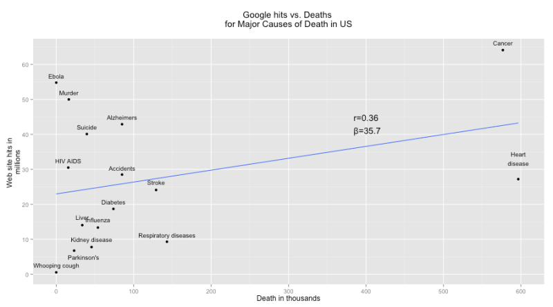
But that’s just an artifact of cancer and heart disease, which kill four times as many Americans as the “runner up,” respiratory diseases.

Once we remove these two, the data shows what I was looking for: presence on the web and mortality have no discernable relationship. In fact, the weak correlation is negative. Respiratory diseases are the number one killer after the cancer and heart disease, but they are not, it seems, web savvy. Same for kidney disease. Anyone have a t-shirt from the “Nephrotic syndrome 5K and Fun Run”? Didn’t think so. And don’t get me started on the flu, the Rodney Dangerfield of infectious diseases. In some cases, the abundance of websites makes sense. HIV AIDS transmission has plummeted becasue of public education. But why is Alzheimer’s a web sensation, whereas stroke is ho-hum? And, in some cases, these mismatches point to dangerous pubic confusion about risk. Heart attacks are considered a “man’s problem” but it’s a major cause of death for women. The relatively weak web presence of heart disease probably flags this gendered misperception, which then leads to the under-diagnosis and under-treatment of women.

Name	Web hits	Deaths	Web search term	CDC term
Ebola	54,800,000	1	Ebola deaths US	Ebola
Whooping cough	549,000	7	Whooping cough deaths US	Whooping cough
HIV AIDS	30,500,000	15,529	HIV AIDS deaths US	Human immunodeficiency virus (HIV) disease
Murder	50,000,000	16,238	Murder deaths US	Assault (homicide)
Parkinson’s disease	6,760,000	23,111	Parkinson’s disease deaths US	Parkinson’s disease
Liver disease	14,050,000	33,642	Liver disease deaths US	Chronic liver disease and cirrhosis
Suicide	40,100,000	39,518	Suicide deaths US	Intentional self-harm (suicide)
Kidney disease	7,780,000	45,591	Kidney disease deaths US	Nephritis, nephrotic syndrome, and nephrosis
Influenza Pnuemonia	13,350,000	53,826	Influenza deaths US PLUS Pnuemonia deaths US	Influenza and Pneumonia
Diabetes	18,700,000	73,831	Diabetes deaths US	Diabetes
Accidents	28,500,000	84,974	Accidents deaths US	Accidents (unintentional injuries)
Alzheimers	42,900,000	84,974	Alzheimer’s deaths US	Alzheimer’s disease
Stroke	24,100,000	128,932	Stroke deaths US	Stroke (cerebrovascular diseases)
Respiratory diseases	9,310,000	142,943	Respiratory disease deaths US	Chronic lower respiratory diseases
Cancer	64,100,000	576,691	Cancer deaths US	Cancer
Heart disease	27,200,000	596,577	Heart disease deaths US	Heart disease

 

 

Visualizing Ebola

The Guardian recently posted a dataviz comparing Ebola to other infectious diseases. It’s from a forthcoming book entitled Knowledge is Beautiful and it is indeed beautiful. Unfortunately, it’s a really bad viz. Below is my alternative viz (using the Guardian’s data), along with a critique.

The basic issue is evolution. Because viruses reproduce quickly so they’re a great example of Darwin at work. Basically a win for a virus is to reproduce a lot. A lot, a lot, a lot. Darwin is simple that way. So once a virus has infected a host, it makes sense to breed like crazy. With one caveat: if you over-reproduce and kill the host, you might lose your transmission vector. So be careful. And if you wait too long, the host might recover: her immune system might learn how to wipe you out. So viruses have to balance virulence and transmission efficiency. You can kill your host quickly, but then you’d better have lots of means of infecting other people. Alternately, if you’re willing to let your host drag around for a week with the sniffles, going to work and school, then you don’t need to be especially infectious. The host will give you plenty of occasions to find new hosts. (I’m blogging with a head cold so this is personal). But overall we should see a clear pattern: more lethal viruses should be more transmissible.

Indeed, my viz below (using the Guardian’s data) shows this rough correlation between virulence and transmissibility. Salmonella doesn’t last long on surfaces, but instead it lets its infected host live and spread the disease through other means. C.diff and tuberculosis are more lethal, but they can survive on surfaces for longer. The Norovirus seems like an outlier, but this makes sense. It spreads primarily through surface contact, so its durability on surfaces is unexpected high. By contrast, Bird Flu is unexpected weak on surfaces, but it spread primarily through droplets. And Ebola is weak on surfaces because it spreads overwhelming through bodily fluid.

But it’s clear that the Guardian’s data is extremely buggy. The data are scraped from the web and are full of errors: HIV does NOT survive on dry surfaces for seven days. That’s probably seven hours. Same for syphilis.

An even bigger problem is that Guardian viz seems to refute Darwin. On their graph deadly diseases seem LESS infectious. What’s going on? First, their x-axis doesn’t make much sense. The reported average rate of infection doesn’t tell us about how well a virus might spread under neutral or ideal conditions. Rather, it tells us how people and public health systems respond to outbreaks. HIV transmission, for example, has dropped in around the world because people have intervened to cut off disease vectors. The difference in HIV prevalence around the world tells us about education, public health, and culture, but not much about the virus itself. Also the x-axis should be on a log scale. And the y-axis should be on a logit scale. Using the fatality rate on a linear scale builds a non-linearity into the relationship, since fatality has to asymptote near 0% and 100%.

So the Guardian graph is indeed beautiful. But it also misuses faulty data to refute evolution. Outside of that it’s great. I’m going to take more ibuprofen now.

 

 

 

 

 

Foodies, sushi, and Google Ngrams

Playing around with the new ngramr package for R, I came up with a simple viz for both the sushi boom and the rise of US foodie culture. Sometime a picture is worth a thousand words, but a least sushi is low in calories.

 

Data illustration vs. data visualization?

Just discovered a great blog post on “data illustration” versus “data visualization” at Information for Humans. AIS argues that data illustration is “for advancing theories” and “for journalism or story-telling.” By contrast data visualization “generate[s] discovery and greater perspective.” I love this distinction, although I’m not sure I like the specific language. Tukey famously argued that data visualization was for developing new theories. Drawing on Tukey, I would use the phrase “exploratory visualization” for techniques that allow us to poke around the data, searching for trends and patterns. Tableau is the great commercial product and Mondrian by Martin Theus is a wonderful freeware application. By contrast, once we have a thesis, we need to convince our audience. That’s “expository data visualization” and it calls for different tools. The R package ggplot2 (http://www.ggplot2.org) is my choice. The terms “expository” versus “exploratory” resonate with freshman comp more that standard data analysis, but that’s the point. After all, this is a DH blog.

Build great models . . . throw them away

The rise of digital humanities suggests the need to rethink some basic questions in quantitative history. Why, for example, should historians use regression analysis? The conventional answer is simple: regression analysis is a social science tool, and historians should use it to do social science history. But that is a limited and constraining answer. If the digital humanities can use quantitative tools such as LDA to complement the close reading of texts, shouldn’t we also have the humanistic use of regression analysis?

What I would like to suggest is idea of model building as a complementary tool in humanistic history, enhancing rather than replacing conventional forms of research. Such an approach rejects what we might call the Time on the Cross paradigm. That approach holds that econometric models are superior to other forms of analysis, and that while qualitative sources might be used to pose questions, on quantitative sources can be used to answer questions. But what if the opposite is true? What if model building can be used to raise questions, which are then answered through texts, or even through archival research?

Let me anchor these ideas in an example: an analysis of the 2012 US News and World report data for college admissions and endowments. Now in a classical social-science history approach, we would first need to posit an explicit hypothesis such as “selective admissions are a linear function of university endowments.” Ideally the hypothesis will involve a causal model, arguing, for example, that undergraduates apply to colleges based on perceived excellence, and that excellence is a result of wealth. Or we might cynically argue that students simply apply to famous schools, and that large endowments increase the applicant pool without any relationship to educational excellence. But humanistic inquiry is better served by an exploratory approach. In exploratory data analysis (EDA) we can start without any formal hypothesis. Instead, we can “get to know the data” and see whether interesting patterns emerge. Rather than proving or disproving a theory, we can treat quantitative data as we would another any other text, searching both for regularities, irregularities, and anomalies.

A basic scatterplot shows an apparent relationship between endowment and the admittance rate: richer schools accept a smaller percentage of their applicants (Figure 1). But the trend is non-linear: there is no limit to endowment, but schools cannot accept less than 0% of their applicants. This non-linearity is simply an artifact of convention. We can understand the data better if we re-express the acceptance rate as ratio of students rejected to students accepted and use a logarithmic scale (Figure 2). There is now a fairly clear trend relating large endowments and high undergraduate admittance rate: the data points track in a broad band from bottom left to top right. But there are also some clear outliers, and examining these leads to interesting insights.

On the left, for example, we find three schools that are markedly more selective than other schools with similar endowments: SUNY College of Environmental Science and Forestry, the University of Georgia, and SUNY Binghamton. On the right is University of Michigan, Ann Arbor. At the bottom are the University of Missouri and University of Iowa. What do these schools have in common? They are all public institutions.

 

When we separate the private and public schools (Figures 3 and 4) it becomes clear that there is no general relationship between endowment and admittance rate. Instead, there is a strong association for private colleges, but almost none for public colleges. These associations are visual apparent: private school fall close to the trend line (a standard OLS regression line), but for public schools the data points form a random cloud. Why? Perhaps the mandate of many state schools is to serve a large number of instate students and that excessively restrictive admissions standards would violate that mandate. Perhaps the quality of undergraduate education is more closely linked to endowment at private schools, so applicants are making a rational decision. Or perhaps, private schools are simply more inclined to game their admittance rate statistics, using promotional materials to attract large numbers of applicants.

What’s striking here is that we no longer need the regression model. The distinction between public and private universities exists as a matter of law. The evidence supporting that distinction is massive and textual. Although we “discovered” this distinction through regression analysis, the details of the model are unnecessary to explain the research finding. In fact, the regression model is vastly underspecified, but that doesn’t matter. It was good enough to reveal that there are two types of university. In fact, the most important regression is the “failure”: the lack of a correlation between endowment and selectivity in public colleges.

So let us image a post-apocalyptic world in which the US university system has been destroyed by for-profit MOOCs and global warming: Harvard, Stanford, and Princeton are underwater both physically and financially, while Michigan Ann Arbor and UI Champaign-Urbana are software products from the media conglomerate Amazon-Fox-MSNBC-Google-Bertelsmann. An intrepid researcher runs a basic regression and discovers that there were once private and public universities. This is a major insight into the lost world of the early twenty-first century. But the research can responsibly present these results without any reference to regression, merely by citing the charters of the school. She might also note that the names of schools themselves are clues to their public-private status. Regression analysis does not supplant close reading, but merely leads our researcher to do close reading in new places.

What’s important here is that these models are, by social science standards, completely inadequate. If we were to seriously engage the question of how endowment drives selectivity we would need to take account of mutual causation: rich schools become selective, but selective schools become rich. That would require combining panel and time series data with some sort of structural model. But we actually don’t need anything that complicated if we are posing questions with models and answering them with qualitative data. In short, we can build a model, then throw it away.

 

 

Back to Basics

Aaron at Plan Space from Outer Nine has a valuable insight about how standard statistics textbooks often favor technique over understanding. I think we could extend approach this from “central tendency” to the broader question of “association.” We tend to view various measures of association  (for example, Chi-square χ², Spearman’s rho ρ, Pearson r, R², etc.) as completely different measurements. But the underlying question is the same: do certain types of values of x tend to coincide with certain values of y? That’s the core question behind most descriptive statistics. The way we measure the association depends on the type of data, but the core question is the same. In data visualization, we can think of mosaic plots and scatterplots as similarly related. How can we see associations in the data? We could use a scatterplot, even for nominal data, but a large coincidence would just result in lots of overplotting. That’s why we use a mosaic plot: association becomes a big box. In short, there is great virtue in returning to first principles

A sensible characterization of mode, median, and mean.